In the last two installments of this series, I showed how we can use Haskell to define a dynamically-sized single-threaded Neural Network and explained things along the way. So yay! We’ve got a Neural Network! Great!

But now that we’ve got it, what in the heck do we do with it? Find out after the cut.

Most Neural Network applications involve defining an initial Neural Network and then fine-tuning the values of each edge by feeding input data into the Neural Network and selecting for Neural Network outputs either manually or by means of an automated process. Artificial Intelligence enthusiasts usually refer to this stage as the evolutionary algorithm, although depending on your usage, training algorithm might be more appropriate. Whichever terminology you choose to prefer, the idea is the same: Reinforce successful outputs and deinforce (is that a word? It is now!) unsuccessful outputs.

Eventually, I’ll be using (a version of) this Neural Network in order to power virtual creatures. Successful Neural Networks will propagate through creature reproduction. Unsuccessful Neural Networks will be weeded out via predation and starvation. Each reproduction will have a chance of mutation, allowing the Neural Network passed on to each new generation to contain slight changes.

But that’ll take a bit more to implement, including a lot of tile map infrastructure, and I really wanted to show something impressive after four posts of, well, theory.

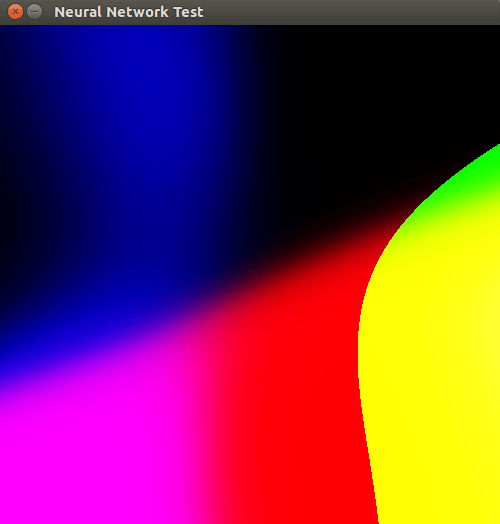
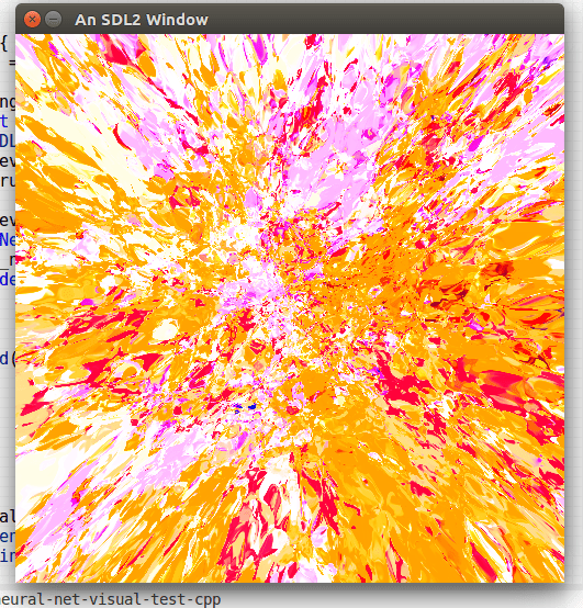
So here’s something else we can do with Neural Networks. We can make pretty pictures!

Okay, so how did I get there?

Some boilerplate application initialization code:

appInit :: IO ()
appInit = do
 initializeAll
 window <- createWindow "Neural Network Test" defaultWindow
 { windowInitialSize = V2 windowWidth windowHeight }
 renderer <- createRenderer window (-1) defaultRenderer
 neural <- buildRandomNeuralNetwork verticeRange [2, 64, 3]
 appLoop neural renderer

Note where I build a random Neural Network on line 7. If we want a Neural Network of a different size, we change the list we pass in there.

The application loop:

appLoop :: NeuralNetwork -> Renderer -> IO ()
appLoop neural renderer = do
 events <- pollEvents
 let eventIsKeyPress key event =
 case eventPayload event of
 KeyboardEvent keyboardEvent ->
 keyboardEventKeyMotion keyboardEvent == Pressed &&
 keysymKeycode (keyboardEventKeysym keyboardEvent) == key
 _ -> False
 keyPressed key = not (null (filter (eventIsKeyPress key) events))
 qPressed = keyPressed KeycodeQ
 rendererDrawColor renderer $= V4 0 0 0 255
 clear renderer
 drawScene neural renderer
 present renderer
 neural' <- mutate verticeRange neural
 unless qPressed $ appLoop neural' renderer

Where things get interesting:

drawScene :: NeuralNetwork -> Renderer -> IO ()
drawScene neural renderer = do
 let generateAllPoints = [(P $ V2 (CInt (fromIntegral x)) (CInt (fromIntegral y))) | x <- [0..(fromIntegral windowWidth)] :: [Int], y <- [0..(fromIntegral windowHeight)]]
 allPoints <- return generateAllPoints
 mapM_ (\point -> drawAnalogOutputForPoint point neural renderer) allPoints

The above code is basically saying for all points on the screen, calculate the Neural Network output for it (which is defined as an RGB color).

Here’s the inner loop’s code:

drawAnalogOutputForPoint :: Point V2 CInt -> NeuralNetwork -> Renderer -> IO ()
drawAnalogOutputForPoint point@(P (V2 (CInt x) (CInt y))) neural renderer = do
outputValues <- return (calculateOutputValues inputs neural)
r <- getOutputValue 0 outputValues
g <- getOutputValue 1 outputValues
b <- getOutputValue 2 outputValues
rendererDrawColor renderer $= V4 r g b 255
drawPoint renderer point
where inputs = [normalizedX, normalizedY]
normalizedX = normalizedDim x windowWidth
normalizedY = normalizedDim y windowHeight
normalizedDim a b = (((fromIntegral a) - (0.5 * (fromIntegral b))) / (fromIntegral b))
normalizeOutput a = floor (a * 256)
getOutputValue n outputValues = return $ normalizeOutput $ outputValues !! n

This is drawing an analog output rather than a winner takes all model. In other words, each value gets red, green, and blue. We could also do a Winner Takes All model, but those pictures tend to be less pretty.

Those pictures above have 69 nodes and 320 edges. About 20% as many nodes (although I’m sure nature has a better implementation than mine) as a roundworm.

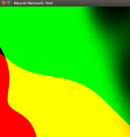
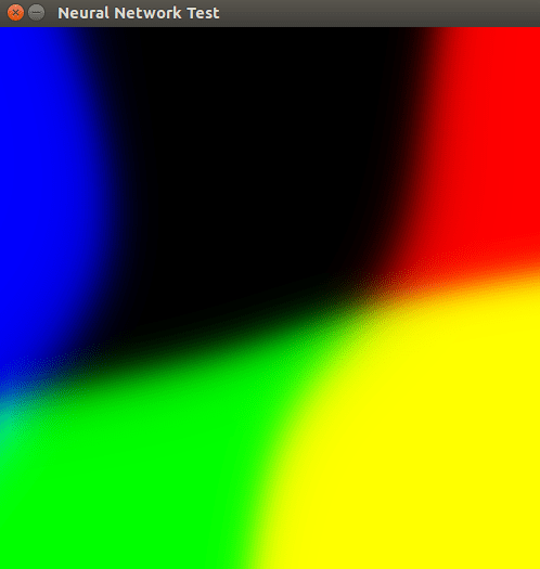
Let’s go more complex. A [2,32,16,8,3] network has eight less nodes, but 728 edges. And more edges means…?

MORE COMPLEX IMAGES!

Keep in mind that these networks are random. Some of them didn’t produce very interesting patterns, so there was a lot of reloading with new networks to get to these neat pictures.

Alright, so what, you might ask. There are less neurons and synapses in this network still than in a roundworm’s nervous system. Show me something IMPRESSIVE, you say, as you sip your morning coffee and get ready to go about your day.

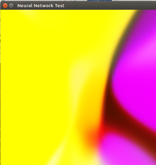
I like a challenge, especially when all I have to do is throw more memory and processor at an existing program to overcome said challenge, so I’ll show you, my discerning internet reader, what happens when we blow things out to 2->1024->512->256->128->64->32->16->8->3. For those of you curious about absolute size, that would be 2045 nodes (40% of a jellyfish) and 701,080 edges. The results? VERY rewarding.

Generating this final image took FAR too long for casual refreshing. I had my computer render it in the background and then came back for it hours later. Luckily, my first shot came out well, because I wanted to end this part of the series with a bang instead of a dull thump.

Thank you for reading with me this far. Next installment, we’ll shift focus from theory and prototypes to performance and implementation. The fun has just begun.